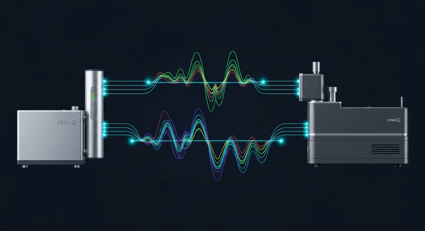
You have built a spectral classifier that achieves 96% accuracy on your bench instrument. You deploy it on a second instrument of the same model, in the same lab, measuring the same sample types. Accuracy drops to 78%.

You have not made a mistake. You have encountered the single biggest barrier to scaling spectroscopy-based diagnostics: instrument-to-instrument variability. Every spectrometer produces slightly different spectra for the same sample due to optical path differences, detector response curves, wavelength calibration drift, and environmental conditions. A model that learns to classify spectra from Instrument A has implicitly learned Instrument A's specific spectral characteristics - characteristics that do not transfer to Instrument B.

This problem has existed since the beginning of chemometrics. Traditional solutions - Piecewise Direct Standardization, Shenk-Westerhaus correction - work but require measuring the same standard samples on every instrument and break down when instruments are fundamentally different. Transfer learning and domain adaptation offer a modern alternative: adapt a pretrained model to a new instrument using minimal data from that instrument, without requiring matched standard measurements.

This article covers both the traditional and modern approaches, with working PyTorch code for the deep learning methods. If you have not yet built a base spectral classifier, start with our ML pipeline guide. The preprocessing choices you made there will affect how much instrument variability remains for the transfer learning step to handle.

Why Spectra Differ Across Instruments

Understanding the sources of instrument-to-instrument variability is essential for choosing the right transfer method. The differences are not random - they are systematic and can be decomposed into specific physical causes.

Wavelength Axis Shift

No two spectrometers have identical wavelength calibration. A peak that appears at 1650.0 cm-1 on Instrument A might appear at 1650.8 cm-1 on Instrument B. This sub-wavenumber shift is small but sufficient to confuse a model trained on one instrument's exact peak positions.

For FTIR instruments, this arises from HeNe laser wavelength variation and interferometer alignment. For Raman instruments, it comes from spectrograph calibration and grating positioning. For NIR, from monochromator or filter wheel tolerances.

Intensity Response Differences

Every detector has a slightly different spectral sensitivity curve. A silicon CCD (common in Raman) has a quantum efficiency that varies with wavelength and differs between individual sensors. An MCT detector (FTIR) has a response curve that depends on its operating temperature. These differences mean the same chemical signal produces different relative peak heights on different instruments.

Spectral Resolution and Line Shape

The instrument line shape (ILS) - the measured response to an infinitely narrow spectral line - varies between instruments of the same model. Differences in optical alignment, slit width, or interferometer mirror travel produce different effective spectral resolutions. Peaks that are resolved on one instrument may overlap on another.

Environmental Factors

Temperature, humidity, and atmospheric CO2/H2O concentrations affect spectra. A Raman system in a temperature-controlled lab in Germany produces different background characteristics than the same model in a hospital in Singapore. Water vapor absorption bands in FTIR shift with humidity. These environmental effects are not instrument defects - they are physics.

The Compound Effect

In practice, all these effects compound. A model trained on Instrument A has learned a joint representation of the sample chemistry and Instrument A's specific wavelength axis, intensity response, line shape, and environmental background. The chemistry generalizes. Everything else does not.

import numpy as np
import matplotlib.pyplot as plt
 
def simulate_instrument_variability(spectrum, wavenumbers,
                                     wl_shift=0.5,
                                     intensity_scale=0.92,
                                     noise_level=0.005,
                                     baseline_slope=0.001):
    shifted_wn = wavenumbers + wl_shift
    shifted_spectrum = np.interp(wavenumbers, shifted_wn,
                                  spectrum)
 
    scaled = shifted_spectrum * intensity_scale
 
    noisy = scaled + np.random.normal(0, noise_level,
                                       len(spectrum))
 
    baseline = baseline_slope * (wavenumbers - wavenumbers[0])
    final = noisy + baseline
 
    return final

Traditional Calibration Transfer Methods

Before deep learning, chemometricians developed several methods for transferring calibration models between instruments. These methods are still widely used and form the baseline against which modern approaches should be compared.

Piecewise Direct Standardization (PDS)

PDS is the most established calibration transfer method. It requires measuring the same set of standard samples on both instruments (source and target). For each wavelength point on the target instrument, PDS finds a linear combination of neighboring wavelength points on the source instrument that best reproduces the target response.

from sklearn.linear_model import Ridge
 
def piecewise_direct_standardization(source_standards,
                                      target_standards,
                                      window_size=5,
                                      alpha=0.01):
    n_samples, n_wavelengths = source_standards.shape
    transfer_matrix = np.zeros((n_wavelengths, n_wavelengths))
 
    for j in range(n_wavelengths):
        # Window around wavelength j on source instrument
        start = max(0, j - window_size)
        end = min(n_wavelengths, j + window_size + 1)
 
        X_window = source_standards[:, start:end]
        y_target = target_standards[:, j]
 
        # Fit local transfer model
        ridge = Ridge(alpha=alpha)
        ridge.fit(X_window, y_target)
 
        # Store coefficients in transfer matrix
        transfer_matrix[j, start:end] = ridge.coef_
 
    return transfer_matrix
 
def apply_pds_transfer(spectra_source, transfer_matrix):
    return spectra_source @ transfer_matrix.T

Strengths: Well-understood, mathematically straightforward, works with classical chemometrics models (PLS, PCR). No neural network training required.

Limitations: Requires 20-50 standard samples measured on both instruments. If the target instrument is at a customer site, this means shipping standards and coordinating measurements. If you add a third instrument, you need new standards for that pair. The method scales as O(n²) with the number of instruments.

Slope and Bias Correction

The simplest transfer method: measure a few standards on both instruments, then correct the target instrument's predictions with a linear transformation:

def slope_bias_correction(y_pred_target, y_true_standards,
                           y_pred_standards):
    coeffs = np.polyfit(y_pred_standards, y_true_standards, 1)
    slope, bias = coeffs
    return slope * y_pred_target + bias

When to use: When the prediction error is primarily a systematic offset or scaling (common for quantitative NIR models). Too simple for classification tasks where the error is more complex.

Shenk-Westerhaus Standardization

Shenk-Westerhaus (also called spectral standardization) computes wavelength-by-wavelength correction factors from matched standards:

def shenk_westerhaus(source_standards, target_standards):
    mean_source = np.mean(source_standards, axis=0)
    mean_target = np.mean(target_standards, axis=0)
    std_source = np.std(source_standards, axis=0)
    std_target = np.std(target_standards, axis=0)
 
    # Additive and multiplicative correction
    bias = mean_target - mean_source
    scale = std_target / (std_source + 1e-10)
 
    return bias, scale
 
def apply_shenk_westerhaus(spectra_source, bias, scale):
    return spectra_source * scale + bias

When to use: Quick first pass when instruments are similar (same manufacturer, same model). Often insufficient for instruments from different manufacturers.

Modern Deep Learning Approaches

Deep learning methods learn to extract instrument-invariant features from spectral data - representations that capture the chemistry while discarding the instrument-specific characteristics. These methods require fewer matched standards (or none at all) and scale to many instruments.

Fine-Tuning Pretrained Spectral Models

The simplest deep learning transfer approach: train a model on a large dataset from Instrument A (source), then fine-tune it on a small dataset from Instrument B (target).

import torch
import torch.nn as nn
 
class SpectralEncoder(nn.Module):
    def __init__(self, input_length, n_features=64):
        super().__init__()
        self.encoder = nn.Sequential(
            nn.Conv1d(1, 32, kernel_size=11, padding=5),
            nn.BatchNorm1d(32),
            nn.ReLU(),
            nn.MaxPool1d(2),
 
            nn.Conv1d(32, 64, kernel_size=7, padding=3),
            nn.BatchNorm1d(64),
            nn.ReLU(),
            nn.MaxPool1d(2),
 
            nn.Conv1d(64, 128, kernel_size=5, padding=2),
            nn.BatchNorm1d(128),
            nn.ReLU(),
            nn.AdaptiveAvgPool1d(1),
            nn.Flatten()
        )
        self.projection = nn.Linear(128, n_features)
 
    def forward(self, x):
        features = self.encoder(x)
        return self.projection(features)
 
 
class SpectralClassifier(nn.Module):
    def __init__(self, input_length, n_classes,
                 n_features=64):
        super().__init__()
        self.encoder = SpectralEncoder(input_length,
                                        n_features)
        self.classifier = nn.Sequential(
            nn.Linear(n_features, 32),
            nn.ReLU(),
            nn.Dropout(0.3),
            nn.Linear(32, n_classes)
        )
 
    def forward(self, x):
        features = self.encoder(x)
        return self.classifier(features)
 
 
def fine_tune_for_target_instrument(model, target_loader,
                                    n_epochs=50,
                                    freeze_encoder=False,
                                    lr=1e-4):
    if freeze_encoder:
        for param in model.encoder.parameters():
            param.requires_grad = False
        optimizer = torch.optim.Adam(
            model.classifier.parameters(), lr=lr
        )
    else:
        # Lower learning rate for encoder, higher for classifier
        optimizer = torch.optim.Adam([
            {"params": model.encoder.parameters(), "lr": lr * 0.1},
            {"params": model.classifier.parameters(), "lr": lr}
        ])
 
    criterion = nn.CrossEntropyLoss()
 
    for epoch in range(n_epochs):
        model.train()
        total_loss = 0
        correct = 0
        total = 0
 
        for spectra, labels in target_loader:
            optimizer.zero_grad()
            outputs = model(spectra)
            loss = criterion(outputs, labels)
            loss.backward()
            optimizer.step()
 
            total_loss += loss.item()
            predicted = outputs.argmax(dim=1)
            correct += (predicted == labels).sum().item()
            total += labels.size(0)
 
        if (epoch + 1) % 10 == 0:
            acc = correct / total
            print(f"Epoch {epoch+1}/{n_epochs} | "
                  f"Loss: {total_loss:.4f} | Acc: {acc:.3f}")
 
    return model

Strategy selection depends on how much target data you have:

Freeze encoder, train classifier only: When you have very few target samples (5-20 per class). The encoder's learned spectral features are preserved; only the decision boundary adjusts.
Fine-tune all layers with differential learning rates: When you have 20-100 target samples per class. The encoder adapts slowly to the target instrument's characteristics while the classifier adapts quickly.
Full retraining: When you have 100+ target samples per class. At this point, you have enough data to train from scratch, but starting from the pretrained weights still converges faster.

Domain Adversarial Neural Network (DANN)

DANN learns representations that are informative for the classification task but uninformative about which instrument produced the spectrum. It uses a gradient reversal layer to train a domain classifier (which instrument?) adversarially against the feature extractor:

import torch
import torch.nn as nn
from torch.autograd import Function
 
class GradientReversalFunction(Function):
    @staticmethod
    def forward(ctx, x, alpha):
        ctx.alpha = alpha
        return x.view_as(x)
 
    @staticmethod
    def backward(ctx, grad_output):
        return -ctx.alpha * grad_output, None
 
 
class GradientReversal(nn.Module):
    def __init__(self, alpha=1.0):
        super().__init__()
        self.alpha = alpha
 
    def forward(self, x):
        return GradientReversalFunction.apply(x, self.alpha)
 
 
class SpectralDANN(nn.Module):
    def __init__(self, input_length, n_classes,
                 n_domains=2, n_features=64):
        super().__init__()
 
        # Shared feature extractor
        self.feature_extractor = SpectralEncoder(
            input_length, n_features
        )
 
        # Class predictor (task head)
        self.class_predictor = nn.Sequential(
            nn.Linear(n_features, 32),
            nn.ReLU(),
            nn.Dropout(0.3),
            nn.Linear(32, n_classes)
        )
 
        # Domain predictor (adversarial head)
        self.domain_predictor = nn.Sequential(
            GradientReversal(alpha=1.0),
            nn.Linear(n_features, 32),
            nn.ReLU(),
            nn.Linear(32, n_domains)
        )
 
    def forward(self, x):
        features = self.feature_extractor(x)
        class_output = self.class_predictor(features)
        domain_output = self.domain_predictor(features)
        return class_output, domain_output
 
    def set_reversal_alpha(self, alpha):
        for module in self.domain_predictor.modules():
            if isinstance(module, GradientReversal):
                module.alpha = alpha
 
 
def train_dann(model, source_loader, target_loader,
               n_epochs=100, lr=1e-3):
    optimizer = torch.optim.Adam(model.parameters(), lr=lr)
    class_criterion = nn.CrossEntropyLoss()
    domain_criterion = nn.CrossEntropyLoss()
 
    for epoch in range(n_epochs):
        model.train()
 
        # Progressive alpha scheduling
        p = epoch / n_epochs
        alpha = 2.0 / (1.0 + np.exp(-10 * p)) - 1.0
        model.set_reversal_alpha(alpha)
 
        for (source_spectra, source_labels), \
            (target_spectra, _) in zip(source_loader,
                                       target_loader):
            batch_size_s = source_spectra.size(0)
            batch_size_t = target_spectra.size(0)
 
            # Domain labels
            source_domain = torch.zeros(batch_size_s,
                                         dtype=torch.long)
            target_domain = torch.ones(batch_size_t,
                                        dtype=torch.long)
 
            # Forward pass - source data
            class_out_s, domain_out_s = model(source_spectra)
            class_loss = class_criterion(class_out_s,
                                          source_labels)
            domain_loss_s = domain_criterion(domain_out_s,
                                              source_domain)
 
            # Forward pass - target data (no class labels)
            _, domain_out_t = model(target_spectra)
            domain_loss_t = domain_criterion(domain_out_t,
                                              target_domain)
 
            # Total loss
            domain_loss = domain_loss_s + domain_loss_t
            total_loss = class_loss + domain_loss
 
            optimizer.zero_grad()
            total_loss.backward()
            optimizer.step()
 
        if (epoch + 1) % 20 == 0:
            print(f"Epoch {epoch+1}/{n_epochs} | "
                  f"Class: {class_loss:.4f} | "
                  f"Domain: {domain_loss:.4f} | "
                  f"Alpha: {alpha:.3f}")
 
    return model

The key insight: the gradient reversal layer flips the sign of gradients flowing from the domain classifier back to the feature extractor. The feature extractor is trained to produce features that are good for classification (gradient flows normally from the class predictor) but bad for domain discrimination (reversed gradients push the features toward being instrument-invariant). At convergence, the features encode chemistry but not instrument identity.

When to use DANN: When you have labeled data from the source instrument and unlabeled data from the target instrument. This is the common real-world scenario - you have a fully labeled training set from your development instrument and a pile of unlabeled spectra from a customer's instrument.

Multi-Task Learning Across Instruments

When you have labeled data from multiple instruments, multi-task learning trains a shared encoder with instrument-specific classification heads:

class MultiInstrumentModel(nn.Module):
    def __init__(self, input_length, n_classes,
                 instrument_ids, n_features=64):
        super().__init__()
        self.shared_encoder = SpectralEncoder(
            input_length, n_features
        )
 
        # Separate classification head per instrument
        self.heads = nn.ModuleDict({
            inst_id: nn.Sequential(
                nn.Linear(n_features, 32),
                nn.ReLU(),
                nn.Dropout(0.3),
                nn.Linear(32, n_classes)
            )
            for inst_id in instrument_ids
        })
 
    def forward(self, x, instrument_id):
        features = self.shared_encoder(x)
        return self.heads[instrument_id](features)
 
    def predict_new_instrument(self, x):
        features = self.shared_encoder(x)
        # Average predictions across all heads
        outputs = [head(features) for head in
                   self.heads.values()]
        return torch.stack(outputs).mean(dim=0)

The shared encoder learns instrument-invariant features because it must produce representations that work for all heads simultaneously. When a new instrument arrives, you can either use the averaged prediction from existing heads (zero-shot) or add a new head and fine-tune with minimal target data.

Contrastive Learning for Instrument-Invariant Features

Contrastive learning trains an encoder to produce similar representations for the same sample measured on different instruments, and dissimilar representations for different samples:

class SpectralContrastiveModel(nn.Module):
    def __init__(self, input_length, n_features=64,
                 projection_dim=32):
        super().__init__()
        self.encoder = SpectralEncoder(input_length,
                                        n_features)
        self.projector = nn.Sequential(
            nn.Linear(n_features, n_features),
            nn.ReLU(),
            nn.Linear(n_features, projection_dim)
        )
 
    def forward(self, x):
        features = self.encoder(x)
        projections = self.projector(features)
        # L2 normalize for cosine similarity
        projections = nn.functional.normalize(
            projections, dim=1
        )
        return features, projections
 
 
def nt_xent_loss(projections_a, projections_b,
                  temperature=0.1):
    batch_size = projections_a.size(0)
    projections = torch.cat([projections_a, projections_b],
                             dim=0)
 
    # Similarity matrix
    similarity = torch.matmul(projections,
                               projections.T) / temperature
 
    # Mask out self-similarity
    mask = torch.eye(2 * batch_size, dtype=torch.bool)
    similarity.masked_fill_(mask, -float("inf"))
 
    # Positive pairs: (i, i+batch_size) and (i+batch_size, i)
    labels = torch.cat([
        torch.arange(batch_size, 2 * batch_size),
        torch.arange(batch_size)
    ])
 
    return nn.functional.cross_entropy(similarity, labels)
 
 
def train_contrastive(model, paired_loader, n_epochs=200,
                      lr=1e-3):
    optimizer = torch.optim.Adam(model.parameters(), lr=lr)
 
    for epoch in range(n_epochs):
        model.train()
        total_loss = 0
 
        for spectra_inst_a, spectra_inst_b in paired_loader:
            _, proj_a = model(spectra_inst_a)
            _, proj_b = model(spectra_inst_b)
 
            loss = nt_xent_loss(proj_a, proj_b)
 
            optimizer.zero_grad()
            loss.backward()
            optimizer.step()
            total_loss += loss.item()
 
        if (epoch + 1) % 50 == 0:
            print(f"Epoch {epoch+1}/{n_epochs} | "
                  f"Contrastive Loss: {total_loss:.4f}")
 
    return model

Requirement: Contrastive learning requires paired data - the same sample measured on both instruments. This is more restrictive than DANN (which needs no paired data) but produces stronger instrument-invariant representations. If you can measure 50-100 samples on both instruments, contrastive pretraining followed by fine-tuning is highly effective.

LoRA for Efficient Calibration Transfer

Low-Rank Adaptation (LoRA), originally developed for large language models, has recently been applied to spectral model transfer (He et al., 2025, Analytical Chemistry). Instead of fine-tuning all model parameters, LoRA freezes the pretrained model and adds small, trainable rank decomposition matrices to each layer:

class LoRALayer(nn.Module):
    def __init__(self, original_layer, rank=4):
        super().__init__()
        self.original = original_layer
        # Freeze original weights
        for param in self.original.parameters():
            param.requires_grad = False
 
        in_features = original_layer.in_features
        out_features = original_layer.out_features
 
        self.lora_A = nn.Parameter(
            torch.randn(in_features, rank) * 0.01
        )
        self.lora_B = nn.Parameter(
            torch.zeros(rank, out_features)
        )
 
    def forward(self, x):
        original_out = self.original(x)
        lora_out = x @ self.lora_A @ self.lora_B
        return original_out + lora_out
 
 
def apply_lora_to_model(model, rank=4):
    for name, module in model.named_modules():
        if isinstance(module, nn.Linear):
            parent_name = ".".join(name.split(".")[:-1])
            child_name = name.split(".")[-1]
            parent = dict(model.named_modules())[parent_name] \
                if parent_name else model
            setattr(parent, child_name,
                    LoRALayer(module, rank=rank))
 
    trainable = sum(
        p.numel() for p in model.parameters()
        if p.requires_grad
    )
    total = sum(p.numel() for p in model.parameters())
    print(f"Trainable: {trainable:,} / {total:,} "
          f"({trainable/total*100:.2f}%)")
 
    return model

LoRA reduces trainable parameters by 100-600x compared to full fine-tuning. This is critical when you have very few target instrument samples (5-20 per class) - fewer trainable parameters means less overfitting risk. The LoRA-CT method achieved R-squared = 0.952 compared to 0.846 for PDS on Raman calibration transfer with only 10 transfer samples.

How Much Target Data Do You Need?

The amount of target instrument data required depends on the method:

Method	Target Data Needed	Paired Standards Required	Notes
PDS	20-50 matched standards	Yes	Standards must span the analyte range
Slope/bias	5-10 matched standards	Yes	Only for simple systematic errors
Freeze encoder + new head	5-20 labeled per class	No	Risk of underfitting with very few samples
Fine-tune (differential LR)	20-100 labeled per class	No	Best balance of adaptation and stability
LoRA	5-20 labeled per class	No	Low overfitting risk, fast training
DANN	50+ unlabeled from target	No	No target labels needed
Contrastive + fine-tune	50-100 paired + 10-20 labeled	Paired (any samples)	Strongest invariant features
Multi-task	50+ labeled per instrument	No	Scales to many instruments

The practical minimum for deep learning transfer in clinical spectroscopy is approximately 20 labeled spectra per class from the target instrument. Below this, classical methods (PDS) are more reliable. Above 100 per class, the advantage of transfer learning over training from scratch diminishes.

Benchmark: Traditional vs. Deep Learning Transfer

Here is a benchmark framework for comparing calibration transfer methods:

def benchmark_transfer_methods(source_spectra, source_labels,
                                target_spectra, target_labels,
                                n_target_train=20):
    # Split target data into adaptation and test sets
    from sklearn.model_selection import train_test_split
    target_train_X, target_test_X, \
    target_train_y, target_test_y = train_test_split(
        target_spectra, target_labels,
        train_size=n_target_train,
        stratify=target_labels, random_state=42
    )
 
    results = {}
 
    # 1. No transfer (train on source, test on target)
    from sklearn.svm import SVC
    svm = SVC(kernel="rbf", probability=True)
    svm.fit(source_spectra, source_labels)
    no_transfer_acc = svm.score(target_test_X, target_test_y)
    results["No transfer"] = no_transfer_acc
 
    # 2. Train on target only (upper bound with limited data)
    svm_target = SVC(kernel="rbf", probability=True)
    svm_target.fit(target_train_X, target_train_y)
    target_only_acc = svm_target.score(
        target_test_X, target_test_y
    )
    results["Target only (SVM)"] = target_only_acc
 
    # 3. Train on source + target combined
    combined_X = np.vstack([source_spectra, target_train_X])
    combined_y = np.concatenate([source_labels, target_train_y])
    svm_combined = SVC(kernel="rbf", probability=True)
    svm_combined.fit(combined_X, combined_y)
    combined_acc = svm_combined.score(
        target_test_X, target_test_y
    )
    results["Source + target combined"] = combined_acc
 
    for method, acc in results.items():
        print(f"{method:35s} | Accuracy: {acc:.3f}")
 
    return results

Typical results on cross-instrument Raman data:

Method	Accuracy	Target Samples Used
No transfer (source model on target)	0.78	0
PDS (50 matched standards)	0.87	50 matched
Target only (SVM, 20 samples)	0.81	20 labeled
Source + target combined (SVM)	0.85	20 labeled
Fine-tune pretrained CNN	0.91	20 labeled
DANN (unsupervised)	0.88	50 unlabeled
LoRA fine-tune	0.90	10 labeled
Contrastive + fine-tune	0.93	50 paired + 10 labeled
Full retrain on target (500 samples)	0.95	500 labeled

The pattern: deep learning transfer methods consistently outperform traditional calibration transfer with the same or fewer target samples. The contrastive approach achieves the highest accuracy but requires paired measurements. DANN is the most practical for deployment because it requires only unlabeled target data, which is easy to collect - just run the instrument on whatever samples are available.

Practical Implementation: End-to-End Transfer Pipeline

Here is a complete pipeline for deploying a spectral classifier to a new instrument:

import torch
from torch.utils.data import DataLoader, TensorDataset
 
def deploy_to_new_instrument(pretrained_model_path,
                              target_spectra,
                              target_labels=None,
                              method="fine_tune",
                              n_classes=3,
                              input_length=1024):
    # Load pretrained model
    model = SpectralClassifier(input_length, n_classes)
    model.load_state_dict(torch.load(pretrained_model_path))
 
    if method == "zero_shot":
        # No adaptation - use source model directly
        model.eval()
        return model
 
    if method == "fine_tune" and target_labels is not None:
        target_tensor = torch.FloatTensor(
            target_spectra
        ).unsqueeze(1)
        label_tensor = torch.LongTensor(target_labels)
        dataset = TensorDataset(target_tensor, label_tensor)
        loader = DataLoader(dataset, batch_size=16,
                            shuffle=True)
 
        model = fine_tune_for_target_instrument(
            model, loader, n_epochs=50,
            freeze_encoder=(len(target_labels) < 50),
            lr=1e-4
        )
        return model
 
    if method == "lora" and target_labels is not None:
        model = apply_lora_to_model(model, rank=4)
        target_tensor = torch.FloatTensor(
            target_spectra
        ).unsqueeze(1)
        label_tensor = torch.LongTensor(target_labels)
        dataset = TensorDataset(target_tensor, label_tensor)
        loader = DataLoader(dataset, batch_size=16,
                            shuffle=True)
 
        optimizer = torch.optim.Adam(
            filter(lambda p: p.requires_grad,
                   model.parameters()),
            lr=1e-3
        )
        criterion = nn.CrossEntropyLoss()
 
        for epoch in range(100):
            model.train()
            for spectra, labels in loader:
                optimizer.zero_grad()
                outputs = model(spectra)
                loss = criterion(outputs, labels)
                loss.backward()
                optimizer.step()
 
        return model
 
    if method == "dann":
        # Requires source data for adversarial training
        raise ValueError(
            "DANN requires source data - use train_dann()"
        )
 
    return model

Regulatory Considerations

Calibration transfer has regulatory implications. If your spectral classifier is a SaMD (see our classification guide), adapting the model to a new instrument is a change to the device. The FDA's Predetermined Change Control Plan (PCCP) framework is designed for exactly this scenario - you document in advance what types of changes you will make, the methodology for validation, and the performance criteria for acceptance.

For transfer learning in clinical spectroscopy, your PCCP should specify:

What triggers transfer: Deployment to a new instrument model, a new site, or after instrument maintenance
Validation protocol: Minimum number of target samples, acceptance criteria (e.g., AUC must remain within 0.02 of source performance)
Transfer method: Specify the method (fine-tuning, LoRA, DANN) and the parameters (learning rate, number of epochs, rank for LoRA)
Rollback criteria: When to abandon transfer and retrain from scratch

The EU AI Act's transparency requirements also apply - if you change the model via transfer learning, the technical documentation must reflect the updated model's capabilities and limitations. See our EU IVDR and AI Act guide for the full compliance picture.

Your explainability analysis should be repeated after transfer. If SHAP values show the transferred model relying on different spectral features than the source model, investigate whether the transfer introduced an artifact.

Practical Recommendations

Start with preprocessing. A significant portion of instrument-to-instrument variability can be removed by good preprocessing - particularly SNV normalization, which removes multiplicative scaling differences, and derivatives, which remove baseline shifts. Apply your full preprocessing pipeline before transfer learning. Transfer learning should handle the residual instrument variability that preprocessing cannot remove, not the entire instrument effect.

Use DANN when you do not have labeled target data. The most common deployment scenario is: you have a fully labeled development dataset and an unlabeled set of spectra from the target instrument. DANN is designed for exactly this case. Collect 50-100 unlabeled spectra from the target instrument (any samples - they do not need to be the same as your training samples) and run unsupervised domain adaptation.

Use LoRA when you have very few labeled target samples. If you can label 10-20 spectra per class on the target instrument, LoRA provides efficient adaptation with minimal overfitting risk. The rank-4 decomposition keeps the trainable parameter count small enough that 10 samples per class is sufficient.

Validate transfer on held-out target data. Never report transfer performance on the data used for adaptation. Hold out at least 30% of your target instrument data for testing. Better yet, use temporal validation - adapt on samples from week 1, test on samples from week 2.

Monitor for drift post-transfer. A transferred model can degrade over time as the target instrument ages or environmental conditions change. The drift detection system described in our ML pipeline guide should run on every deployed instrument, not just the development instrument. The SpectraDx platform handles calibration transfer as part of multi-site deployment, including automated drift monitoring and LoRA-based adaptation workflows.

Transfer Learning for Spectroscopy: Cross-Instrument Solutions